Hash Length of SHA 265

It is important to note that any hash algorithm always returns a hash of fixed length. 

SHA256 returns a hash value that is 256 bits - i.e. 32 bytes. 

These 32 bytes are typically represented as a hexademical string of 64 bytes. 

Hence to store a SHA256 hash, we just need 64 bytes (in database terms - varchar(64)).

Does Bitcoin encrypt transactions?

 *It is important to note that the core bitcoin network/ledger does not use any encryption. It is all hashing as explained here - https://www.narendranaidu.com/2022/05/ruminating-on-proof-of-work.html 

But each and every transaction is digitally signed by a user (or wallet). 

Hence a bitcoin network uses digital signatures and as we know a digital signature is nothing but an encrypted hash of the data. 

You can digitally sign any data in the following way (creating an encrypted hash of the data)

• Hash the data using SHA-256.
• Encrypt the generated hash using your private key. 
• Package this encrypted hash and your public key together. 

The public key is part of the digital signature, whereas the private key is securely stored in a digital wallet (never to be shared with anyone). 

In the bitcoin network, this digital signature is created using the Elliptic Curve Digital Signature Algorithm (ECDS). ECC encryption is not used! - Many folks get confused by this :)

Ruminating on Elliptic Curve Cryptography

When it comes to symmetric encryption, the most common standards are Data Encryption Standards (DES) and Advanced Encryption Standards (AES).

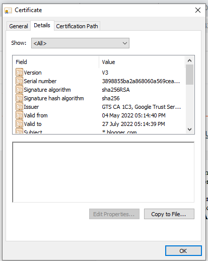
When it comes to asymmetric encryption (public key cryptography), the dominant standard is  RSA (Rivest-Shamir-Adleman). Almost all the digital certificates (HTTPS/SSL) issued used RSA as the encryption standard and SHA256 as the hashing algorithm. 

Given below is a screenshot of a digital certificate of a random HTTPs site. You can see the encryption algorithm and Hash function mentioned in the certificate. 

There is another asymmetric encryption standard called as ECC (Elliptic Curve Cryptography) that is very popular in the crypto world. 

ECC has the following advantages when compared to RSA:

• It can run on low end devices (low CPU and memory).
• It is faster - for both encryption/decryption.
• Smaller key size - 256-bit elliptic curve private key is just as secure as a 3072-bit RSA private key. Smaller keys are easier to manage and work with.

While certificate issuers have started providing ECC standard based digital certificates, it is important to note that not all browsers (mobile, desktop) still support it. Also a lot of legacy apps may not have support for ECC standard and these have to be refactored for SSL to work again. 

Ruminating on Proof of Work

While I understood how bitcoin mining worked, there were still a few strings loose in my mind on why exactly was the 'Proof-of-Work' algorithm created that way? (i.e. finding a nonce that results in a hash lower than the target value)

The following video from Khan Academy gives an excellent understanding of PoW is very simple terms - https://www.khanacademy.org/economics-finance-domain/core-finance/money-and-banking/bitcoin/v/bitcoin-proof-of-work

Also the following snippets from Investopedia: https://www.investopedia.com/terms/n/nonce.asp would give a better idea on the challenge (finding the right nonce) that all bitcoin miners are trying to solve. 

"A nonce is an abbreviation for "number only used once," which, in the context of cryptocurrency mining, is a number added to a hashed—or encrypted—block in a blockchain that, when rehashed, meets the difficulty level restrictions. The nonce is the number that blockchain miners are solving for. When the solution is found, the blockchain miners are offered cryptocurrency in exchange.

A target hash is a numeric value that a hashed block header (which is used to identify individual blocks in a blockchain) must be less than or equal to in order for a new block to be awarded to a miner.

The Bitcoin network adjusts the difficulty of mining by raising or lowering the target hash in order to preserve an average 10-minute interval between new blocks.

The block header contains the block version number, a timestamp, the hash used in the previous block, the hash of the Merkle Root, the nonce, and the target hash. The block is generated by taking the hash of the block contents, adding a random string of numbers (the nonce), and hashing the block again.

Determining which string to use as the nonce requires a significant amount of trial-and-error, as it is a random string. A miner must guess a nonce, append it to the hash of the current header, rehash the value, and compare this to the target hash. If the resulting hash value meets the requirements (golden nonce), the miner has created a solution and is awarded the block.

It is highly unlikely that a miner will successfully guess the nonce on the first try, meaning that the miner may potentially test a large number of nonce options before getting it right. The greater the difficulty—a measure of how hard it is to create a hash that is less than the target—the longer it is likely to take to generate a solution."

Ultimately it is all about guessing a nonce and calculating the hash and comparing it. Hence the capacity of a bitcoin mining farm is calculated in terms of hash rate - i.e. number of hashes that can be computed per second. The term 'Bitcoin mining' is actually misleading as what the miners are actually doing is finding a hash that satisfies the challenge and this also validates the transactions in the block (and the block gets added to the chain). 

But as many miners jump on the bandwagon, there is lot of wastage of compute cycles and this is a controversial topic for many people.  

Numeric value of a hash

In the bitcoin network, miners have to compare the hash value during the 'Proof-of-Work' process.

The target hash value is stored in the header and is expressed as a 67-digit number. Miners must find a new hash of the transaction block  that is below the given target. 

To solve the hash puzzle, miners will try to calculate the hash of a block by adding a nonce to the block header repeatedly until the hash value yielded is less than the target.

But how is the value of the hash calculated? In the bitcoin network, the value of a hash is calculated as follows:

• Hashes are typically represented as a hexadecimal string. Convert the hexadecimal value to decimal value. 
• Get the base-2 log of the decimal value. 

This is the value that is compared against the target in the block header. 

Ruminating on dedicated instance vs. dedicated host

 Many folks get confused between the AWS terminology of 'Dedicated Instance' vs 'Dedicated Host'.

A simple way to understand the difference is to remember that a "host" is a physical machine that can host many virtual machine instances. 

Hence a "dedicated host" is a physical machine that is dedicated to your organization. On this physical machine (host), you can install many VMs/containers. So you control what VMs (instances) are going to run on that host. 

So what is a dedicated instance then? A dedicated instance is a virtual machine that runs on hardware that is not shared with other accounts. Dedicated instances are physically isolated at the host hardware level from instances that belong to other AWS accounts. Hence you can only be certain that the underlying hardware that is hosting your VM is not shared with someone else. But you have no fine-grained control over which VM would be launched on which host, etc. 

Cloud Native Banking Platform - Temenos

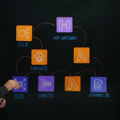
Temenos is the world's number one core banking platform. It is built entirely on the AWS cloud and uses all managed services. 

I was stuck with the simplicity of the overall architecture on AWS and how it enabled elastic scalability to scale-out for peak loads and also scale-back for reducing operational costs. 

Another interesting aspect was the simple implementation of the CQRS pattern to offload queries (read-only API requests) to DynamoDB. The pipeline was built using Kinesis and Lambda. 

An excellent short video on the AWS architecture of the Temenos platform is here: https://youtu.be/mtZvA7ARepM

Difference between Epoch, Batch and Iterations

In neural nets, we have to specify the number of epochs while we train the model. 

One Epoch is defined as the complete forward & backward pass of the neural net over the complete training dataset. We need to remember that Gradient Descent is an iterative process and hence we need multiple passes (or epochs) to find the optimal solution. In each epoch, the weights and biases are updated. 

Batch size is the number of records in one batch. One Epoch may consist of multiple batches. The training dataset is split into batches because of memory space requirements. A large dataset cannot be fit into memory all at once. With increase in Batch size, required memory space increases. 

Iterations is the number of batches needed to complete one epoch. So if we have 2000 records and a batch size of 500, then we will need 4 iterations to complete one epoch. 

If the number of epochs are low, then it results in underfitting the data. As the number of epochs increases, more number of times the weight are changed in the neural network and the curve goes from underfitting to optimal to overfitting curve. Then how do we determine the optimal number of epochs?

It is done by splitting the training data into 2 subsets - a) 80% for training the neural net  b) 20% for validating the model after each epoch. The fundamental reason we split the dataset into a validation set is to prevent our model from overfitting. The model is trained on the training set, and, simultaneously, the model evaluation is performed on the validation set after every epoch.

Then we use something called as the "early stopping method"-  we essentially keep training the neural net for an arbitrary number of epochs and monitor the performance on the validation dataset after each epoch. When there is no sign of performance improvement on your validation dataset, you should stop training your network. This helps us arrive at the optimal number of epochs. 

A good explanation of these concepts is available here - https://www.v7labs.com/blog/train-validation-test-set. Found the below illustration really useful to understand the split of data between train/validate/test sets. 

Ruminating on Convolutional Neural Networks

Convolutional Neural Nets (CNNs) have made Computer Vision a reality. But to understand CNNs, we need to get basics right - What exactly is a convolution? What is a kernel/filter?

The kernel or filter is a small matrix that is multiplied by the source image matrix to extract features. So you can have a kernel that identifies edges or corners of a photo. Then there could be kernels that detect patterns - e.g. eyes, stripes.

A convolution is a mathematical operation where a kernel (aka filter) moves across the input image and does a dot product of the kernel and the original image. This dot product is saved as a new matrix and is called as the feature map. An excellent video visualizing this operation is available here - https://youtu.be/pj9-rr1wDhM

Image manipulation software such as Photoshop also use kernels for effects such as 'blur background'. 

One fundamental advantage of the convolution operation is that if a particular filter is designed to detect a specific type of feature in the input, then applying that filter systematically across the entire input image allows us to discover that feature anywhere in the image. Also note that a particular convolutional layer can have multiple kernels/filters. So after the input layer (a single matrix), the convolutional layer (having 6 filters) will produce 6 output matrices. A cool application to visualize this is here - https://www.cs.ryerson.ca/~aharley/vis/conv/flat.html

A suite of tens or even hundreds of other small filters can be designed to detect other features in the image. After a convolutional layer, we also typically add a pooling layer. Pooling layers are used to downsize the features maps - keeping the important parts and discarding the rest. The output matrices of the pooling layer are smaller in size and faster to process. 

So as you can see, the fundamental difference between a densely connected layer and a convolutional layer is that dense fully connected layers learn global patterns (involving all pixels) whereas convolution layers learn local features (edges, corners, textures, etc.) 

Using CNNs, we can create a hierarchy of patterns - i.e. the second layer learns from the first layer. CNNs are also reusable, so we can take an image classification model trained on https://www.image-net.org/ dataset and add additional layers to customize it for our purpose. 

A good introduction to CNN models is given in this article - https://towardsdatascience.com/convolution-neural-networks-a-beginners-guide-implementing-a-mnist-hand-written-digit-8aa60330d022 with a good PyTorch implementation for MNIST dataset here - https://towardsdatascience.com/mnist-handwritten-digits-classification-using-a-convolutional-neural-network-cnn-af5fafbc35e9

Ruminating on Activation Function

 Activation functions play an important role in neural nets. An activation function transforms the weighted sum of the input into an output from a node. 

Simply put, an activation function defines the output of a neuron given a set of inputs. It is called "activation" to mimic the working of a brain neuron. Our neurons get activated due to some stimulus. Similarly the activation function will decide which neurons in our neural net get activated. 

Each hidden layer of a neural net needs to be assigned an activation function. Even the output layer of a neural net would use an activation function. 

The ReLU (Rectified Linear Unit) function is the most common function used for activation. 

The ReLU function is a simple function: max(0.0, x). So essentially it takes the max of either 0 or x. Hence all negative values are ignored. 

Other activation functions are Sigmoid and Tanh. The sigmoid activation function generates an output value between 0 and 1. 

An excellent video explaining activation function is here - https://youtu.be/m0pIlLfpXWE

The activation functions that are typically used for the output layer are Linear, Sigmoid (Logistic) or Softmax. A good explanation of when to use what is available here - https://machinelearningmastery.com/choose-an-activation-function-for-deep-learning/

Ruminating on Gradient Descent

Gradient Descent is the most popular optimization algorithm used to train machine learning models - by minimizing the cost function. In deep learning, neural nets use back-propagation that internally use a cost function (aka lost function) like Gradient Descent. 

The Gradient descent function essentially uses calculus to find the direction of travel and then to find the local minimal of a function. The following 2 videos are excellent tutorials to understand Gradient Descent and their use in neural nets. 

https://youtu.be/IHZwWFHWa-w

https://youtu.be/sDv4f4s2SB8

Once you understand these concepts, it will help you also realize that there is no magic involved when a neural net learns by itself -- ultimately a neural net learning by itself just means minimizing a cost function (aka loss function).

Neural nets start with random values for their weights (of the channels) and biases. Then by using the cost function, these hundreds of weights/biases are shifted towards the optimal value - by using optimization techniques such as gradient descent. 

Ruminating on 'Fitting the line to data'

 In linear regression, we need to find the best fit line over a set of points (data). StatQuest has an excellent video explaining how we fit a line to the data using the principle of 'least squares' - https://www.youtube.com/watch?v=PaFPbb66DxQ

The best fit line is the one where the sum of the squares of the distances from the actual points to the line is the minimum. Hence this becomes an optimization problem in Maths that can be calculated. We square the distances to take care of negative values/diffs. 

In stats, the optimization function that minimizes the sum of the squared residuals is also called as a 'loss function'. 

The equation of any line can be stated as: y = ax + b

where a is the slope of the line and b is the y-intercept. Using derivates we can find the most optimal values of 'a' and 'b' for a given dataset. 

Ruminating on CUDA and TPU

 CUDA  is a parallel computing platform (or a programming model - available as an API) that was developed by Nvidia to enable developers leverage the full parallel processing power of its GPUs. 

For deep learning (training neural nets) requires a humongous amount of processing power and it is here that HPCs with thousands of GPU cores (e.g. A100 GPU) are essential. 

Nvidia has also released a library for use in neural nets called as cuDNN. CUDA Deep Neural Network library (cuDNN) is a GPU-accelerated library of primitives for deep neural networks. cuDNN provides highly tuned implementations for standard routines such as forward and backward convolution, pooling, normalization, and activation layers.

Many deep learning frameworks rely on CUDA & the cuDNN library for parallelizing work on  GPUs - Tensorflow, Caffe2, H2O.ai, Keras, PyTorch. 

To address the growing demand for training ML models, Google came up with it's own custom integrated circuit called as TPU (Tensor Processing Unit). A TPU is basically a ASIC (application-specific integrated circuit) designed by Google for use in ML. TPU's are tailored for TensorFlow and can handle massive multiplications and additions for neural networks, at great speeds while reducing the use of too much power and floor space. 

Examples: Google Photos use TPU's to process more than 100 million photos every day. TPU's also power Google RankBrain - that part of Google's algorithm that uses machine-learning and artificial intelligence to better understand the intent of a search query. 

Understanding what is a Tensor?

Found this excellent video on YouTube by Prof. Daniel Fleisch that explains tensors in a very simple and engaging way - https://youtu.be/f5liqUk0ZTw

Tensors are are generalizations of vectors & matrices to N-dimensional space.

• A scalar is a 0 dimensional tensor
• A vector is a 1 dimensional tensor
• A matrix is a 2 dimensional tensor
• A nd-array is an N dimensional tensor

The inputs, outputs, and transformations within neural networks are all represented using tensors.  A tensor can be visualized as a container which can house data in N dimensions.

Topic Modeling vs. Topic Classification

Topic Modeling is an unsupervised method of infering "topics" or classification tags within a cluster of documents. Whereas topic classification is a supervised ML approach wherein we define a list of topics and label a few documents with these topics for training. 

A wonderful article explaining the differences between both the approaches is here - https://monkeylearn.com/blog/introduction-to-topic-modeling/

Some snippets from the above article:

"Topic modeling involves counting words and grouping similar word patterns to infer topics within unstructured data. By detecting patterns such as word frequency and distance between words, a topic model clusters feedback that is similar, and words and expressions that appear most often. With this information, you can quickly deduce what each set of texts are talking about.

 If you don’t have a lot of time to analyze texts, or you’re not looking for a fine-grained analysis and just want to figure out what topics a bunch of texts are talking about, you’ll probably be happy with a topic modeling algorithm.

However, if you have a list of predefined topics for a set of texts and want to label them automatically without having to read each one, as well as gain accurate insights, you’re better off using a topic classification algorithm."

Ruminating on the log scale

Today, I was trying to explain my colleague on the usecases where a log scale could be more useful than a linear scale and I found this wonderful video that explains this concept like a boss! - https://youtu.be/eJF9hiv3c-A

One of the fundamental advantages of using the log scale is that you can illustrate both small and large values on the same graph. Log scales are also consistent because each unit increase signifies the same multiplier effect - e.g. Log10 has 10* multiplier. 

I also never knew the following scales used popularly are actually log scales:

• Audio volume (decibel) - 10x increase from 50 decibel to 60 decibel
• Acidity (ph scale)
• Richter scale (earthquakes)
• Radioactivity (measure of radiation)

Ruminating on AI Knowledge Base

Many AI systems need a knowledge base that enables logical inference over the knowledge stored in it. This knowledge base is typically encoded using open standards such as RDF (Resource Description Framework).  

To read RDF file, we typically use SPARQL - which is an RDF query language—that is, a semantic query language for databases—able to retrieve and manipulate data stored in RDF. 

A simple Python library to use SPARQL - https://sparqlwrapper.readthedocs.io/

Also some other helper classes if you are not comfortable with SPARQL - https://github.com/qcri/RDFframes

Other popular datastores that support RDF formats are GraphDB and Neo4J

The best example of a knowledge base (or graph) is the "Google Knowledge Graph" - a knowledge base used by Google and its services to enhance its search engine's results with information gathered from a variety of sources. The information is presented to users in an infobox next to the search results.

Ruminating on Audio Sample Rate and Bit Depth

 Whenever we are dealing with AI-driven speech recognition, it is important to understand the fundamental concepts of sample rate and bit dept. The following article gives a good overview with simple illustrations. 

https://www.izotope.com/en/learn/digital-audio-basics-sample-rate-and-bit-depth.html

To convert a sound wave into data, we have to measure the amplitude of the wave at different points of time. The number of samples per second is called as the sample rate. So a sample rate of 16kHz means 16,000 samples were taken in one second. 

The bit depth determines the number of possible amplitude values we can record for each sample - e.g. 16-bit, 24-bit, and 32-bit. With a higher audio bit depth, more amplitude values are available for us to record. The following diagram form the above article will help illustrating this concept. 

Free audiobooks

The below site has more than 16,000 audio books that are completely free for everyone!

https://librivox.org/

Would recommend everyone to check this out. 

Ruminating on the Turing Test

 The Turing Test was made famous by Alan Turing in the year 1950. The Turing Test essentially tests a computer's ability to communicate indistinguishably from a human. The Turing Test was also called as the 'Imitation Game' by Alan earlier. 

A good introduction to the Turing Test can be found here - https://youtu.be/3wLqsRLvV-c

Though many claim that the turing test was passed by a AI chatbot called Eugene Goostman, but in reality it is not so. No computer has ever passed the Turing Test - https://isturingtestpassed.github.io/

Intelligent chatbots have really come a long way - The Google Duplex Demo e.g. https://youtu.be/0YaAFRirkfk

Maybe when we achieve AGI (Artificial General Intelligence), then the Turing Test would be accurately passed :)

Ruminating on n-gram models

N-gram is a fundamental concept in NLP and is used in many language models. In simple terms, N-gram is nothing but a sequence on N words - e.g. San Francisco (is a 2-gram) and The Three Musketeers (is a 3-gram). 

N-grams are very useful because they can be used for making next word predictions, correcting spellings or grammar. Ever wondered how Gmail is able to suggest auto-completion of sentences? This is possible because Google has created a language model that can predict next words.

N-grams are also used for correcting spelling errors - e.g. “drink cofee” could be corrected to “drink coffee” because the language model can predict that 'drink' and 'coffee' being together have a high probability. Also the 'edit distance' between 'cofee' and 'coffee' is 1, hence it is a typo.

Thus N-grams are used to create probabilistic language models called n-gram models. N-gram models predict the occurrence of a word based on its N – 1 previous word. 

The 'N' depends on the type of analysis we want to do - e.g. Research has also shown that trigrams and 4-grams work the best for spam filtering. 

Some good info on N-grams is available at the Standford University site - https://web.stanford.edu/~jurafsky/slp3/slides/LM_4.pdf

Google books also has a "N-Gram" viewer displays a graph showing how those phrases have occurred in a corpus of books (e.g., "British English", "English Fiction", "French") over the selected years. I found this to be useful in understanding what topic was popular in which years: https://books.google.com/ngrams

Ruminating on Text Normalization

Text normalization is the process of converting text to a standard form before we use them for training AI NLP models. The following techniques are typically used for normalizing text. 

Tokenization:  Tokenization is the process of breaking down sentences into words. In many Latin-derived languages, "space" is considered to be a word delimeter. But there are special cases such as 'New York', 'Rock-n-Roll' etc. Also Chinese and Japanese languages do not have spaces between words. We may laso wante to tokenize emoticons and hashtags. 

Lemmatization: In this process, we check if words have the same 'root' - e.g. sings, sang. We then normalize the words to the common root word. 

Stemming: Stemming can be considered a form of Lemmatization wherein we just strip the suffixes from the end of the word - e.g. troubled and troubles can be stemmed to 'troubl'.

Lemmatization is more computationally intensive than Stemming because it actually maps the word to a dictionary and finds the root word. Whereas Stemming just uses some crude heuristic process that chops off the ends of words in the hope of getting the root word. Stemming is thus much faster when you are dealing with a large corupus of text. The following examples will make the difference clear. 

• The word "better" has "good" as its lemma. This link is missed by stemming, as it requires a dictionary look-up.
• The word "walk" is the base form for word "walking", and hence this is matched in both stemming and lemmatisation.
• If you lemmatize the word 'Caring', it would return 'Care'. If you stem, it would return 'Car' and this is erroneous.

Sentence Segmentation: This entails breaking up a long sentence into smaller sentences using chars such as '! ; ?'. 

Spelling Correction and UK/US differences: As part of the normalization activity, we may also want to correct some common spelling mistakes and also normalize the different spelling between UK/US like neighbour/neighbor.

Ruminating on Fourier Transformation

 In my AI learning journey, I had to refresh my understanding of fourier transformation. The following video on YouTube is hands-down the best tutorial for understanding this maths concept.

Fourier transformations are used in AI Computer Vision models for usecases such as edge detection, image filtering, image reconstruction, and image compression. 

Fuzzy matching of Strings

Quite often during document processing or email processing tasks, we need to compare strings or search for keywords. While the traditional way of doing this would be using String comparison or RegEx, there are a number of other techniques available. 

Fuzzy matching is an approximate string matching technique that is typically used to identify typos or spelling mistakes. Fuzzy matching algorithms try to measure how close two strings are to one another using a concept called as 'Edit Distance'. In simple words, 'edit distance' can be considered as the number of edits required to make both the sentences same. There are different types of edit distance measurements as described in the Wikipedia article above. 

TheFuzz is a cool Python library that can be used to measure the Levenshtein Distance between sequences. The following articles would help you quickly grasp the basics of using the library. 

https://www.activestate.com/blog/how-to-implement-fuzzy-matching-in-python/

https://www.analyticsvidhya.com/blog/2021/07/fuzzy-string-matching-a-hands-on-guide/

https://towardsdatascience.com/fuzzy-string-matching-in-python-68f240d910fe

Ruminating on Snowflake Architecture

 The following video is an excellent tutorial to understand how Snowflake can perform both as a Data Lake and Datawarehouse.

https://www.youtube.com/watch?v=jmVnZPeClag

The following articles on Snowflake are also worth a perusal:

https://www.snowflake.com/workloads/data-warehouse-modernization/

https://www.snowflake.com/guides/data-lake

The following key concepts are important to understand to appreciate how Snowflake works:

• Snowflake separates compute with storage and each can be scaled out independently
• For storage, Snowflake leverages distributed cloud storage services like AWS S3, Azure Blob, Google Cloud Storage). This is cool since these services are already battle-tested for reliability, scalability and redundancy. Snowflake compresses the data in these cloud storage buckets. 
• For compute, Snowflake has a concept called as "Virtual warehouse". A virtual warehouse is a simple bundle of compute (CPU) and memory (RAM) with some temperory storage. All SQL queries are executed in the virtual warehouse. 
• Snowflake can be queried using plain simple SQL - so no specialized skills required. 
• If a query is fired more frequently, then the data is cached in memory. This "Cache" is the magic that enables fast ad-hoc queries to be run against the data. 
• Snowflake enables a unified data architecture for the enterprise since it can be used as a Data Lake as well as a Data warehouse. The 'variant' data type can store JSON and this JSON can also be queried. 

The virtual datawarehouse provide a kind of dynamic scalability to the Snowflake DW. Snippets from the Snowflake documentation.

"The number of queries that a warehouse can concurrently process is determined by the size and complexity of each query. As queries are submitted, the warehouse calculates and reserves the compute resources needed to process each query. If the warehouse does not have enough remaining resources to process a query, the query is queued, pending resources that become available as other running queries complete. If queries are queuing more than desired, another warehouse can be created and queries can be manually redirected to the new warehouse. In addition, resizing a warehouse can enable limited scaling for query concurrency and queuing; however, warehouse resizing is primarily intended for improving query performance. 

With multi-cluster warehouses, Snowflake supports allocating, either statically or dynamically, additional warehouses to make a larger pool of compute resources available". 

Ruminating on Joint Probability vs Conditional Probability vs Marginal Probability

The concept of conditional probability is a very important to understand Bayesian networks. An excellent introduction to these concepts is available in this video - https://youtu.be/5s7XdGacztw

As we know, probability is calculated as the number of desired outcomes divided by the total possible outcomes. Hence if we roll a dice, the probability that it would be 4 is 1/6 ~ (P = 0.166 = 16.66%)

Siimilary, the probability of an event not occurring is called as the complement ~ (1-P). Hence the probability of not rolling a 4 would = 1-0.166 = 0.833 ~ 83.33%

While the above is true for a single variable, we also need to understand how to calculate the probability of two or more variables - e.g. probability of lightening and thunder happening together when it rains. 

When two or more variables are involved, then we have to consider 3 types of probability:

1) Joint probability calculates the likelihood of two events occurring together and at the same point in time. For example, the joint probability of event A and event B is written formally as:  P(A and B) or  P(A ^ B) or P(A, B)

2) Conditional probability measures the probability of one event given the occurrence of another event.  It is typically denoted as P(A given B) or P(A | B). For complex problems involving many variables, it is difficult to calculate joint probability of all possible permutations and combinations. Hence conditional probability becomes a useful and easy technique to solve such problems. Please check the video link above. 

3) Marginal probability is the probability of an event irrespective of the outcome of another variable.

Another excellent article explaining conditional probability with real life examples is here - https://www.investopedia.com/terms/c/conditional_probability.asp 

Confusion Matrix for Classification Models

Classification models are supervised ML models used to classify information into various classes - e.g. binary classification (true/false) or multi-class classification (facebook/twitter/whatsapp)

When it comes to classification models, we need a better metric than accuracy for evaluating the holistic performance of the model. The following article gives an excellent overview of Confusion Matrix and how it can be used to evaluate classification models (and also tune their performance).

https://www.analyticsvidhya.com/blog/2020/04/confusion-matrix-machine-learning/

Some snippets from the above article:

A Confusion matrix is an N x N matrix used for evaluating the performance of a classification model, where N is the number of target classes. The matrix compares the actual target values with those predicted by the machine learning model. This gives us a holistic view of how well our classification model is performing and what kinds of errors it is making.

A binary classification model will have false positives (aka Type 1 error) and false negatives (aka Type 2 error). A good example would be a ML model that predicts whether a person has COVID based on symptoms and the confusion matrix would look something like the below. 

Based on the confusion matrix, we can calculate other metrics such as 'Precision' and 'Recall'. 

Precision is a useful metric in cases where False Positive is a higher concern than False Negatives.

Recall is a useful metric in cases where False Negative trumps False Positive.

Recall is important in medical cases where it doesn’t matter whether we raise a false alarm but the actual positive cases should not go undetected!

F1-score is a harmonic mean of Precision and Recall, and so it gives a combined idea about these two metrics. It is maximum when Precision is equal to Recall.

Another illustration of a multi-class classification confusion matrix that predicts the social media channel. 

Bias and Variance in ML

Before we embark on machine learning, it is important to understand basic concepts around bias, variance, overfitting and underfitting. 

The below video from StatQuest gives an excellent overview of these concepts: https://youtu.be/EuBBz3bI-aA

Another good article explaining the concepts is here - https://towardsdatascience.com/understanding-the-bias-variance-tradeoff-165e6942b229

Bias as the difference (aka error) between the average prediction made by the ML model and the real data in the training set. The bias shows how well the model matches the training dataset. A low bias model will closely match the training data set. 

Variance refers to the amount by which the predictions would change if we fit the model to a different training data set. A low variance model will produce consistent predictions across different datasets. 

Ideally, we would want a model with both a low bias and low variance. But we often need to do a trade-off between bias and variance. Hence we need to find a sweet spot between a simple model and a complex model. 

Overfitting means your model has a low bias but a high variance. It overfits the training dataset. 

Underfiting means your model has a high bias but a low variance. 

If our model is too simple and has very few parameters then it may have high bias and low variance (underfitting). On the other hand if our model has large number of parameters then it’s going to have high variance and low bias (overfitting). So we need to find the right/good balance without overfitting and underfitting the data.

Ruminating on high dimensional data

 In simple terms, dimensions of a dataset refer to the number of attributes (or features) that a dataset has. This concept of dimensions of data is not new and quite common in the data warehousing world as explained here. 

Many datasets can have a large number of features (variables/attributes) such as healthcare data, signal processing, bioinformatics. When the number of dimensions are staggeringly high, ML calculations become extremely difficult. It is also possible that the number of features can exceed the number of observations (or records in a dataset) - e.g. microarrays, which measure gene expression, can contain hundreds of samples/records, but each record can contain tens of thousands of genes.

In such highly dimensional data, we experience something called as the "Curse of dimensionality" - i.e. all records appear to be sparse and dissimilar in many ways, which prevents common data organization strategies from being efficient. The more dimensions we add to a data set, the more sparse the data becomes and this results in an exponential decrease in the ML model performance (i.e. predictive capabilities). 

A typical rule of thumb is that there should be at least 5 training examples for each dimension in the dataset. Another interesting excerpt from Wikipedia is given below:   

In machine learning and insofar as predictive performance is concerned, the curse of dimensionality is used interchangeably with the peaking phenomenon, which is also known as Hughes phenomenon. This phenomenon states that with a fixed number of training samples, the average (expected) predictive power of a classifier or regressor first increases as the number of dimensions or features used is increased but beyond a certain dimensionality it starts deteriorating instead of improving steadily.

To handle high dimensional datasets, data scientists typically perform various data dimension reduction techniques on the datasets - e.g. feature selection, feature projection, etc. More information about dimension reduction can be found here. 

Ruminating on ONNX format

Open Neural Network Exchange (ONNX) is an open standard format for representing machine learning models. While there are proprietary formats such as pickle (for Python) and MOJO (for H20 AI), there was a need to drive interoperability. 

ONNX defines a common set of operators - the building blocks of machine learning and deep learning models - and a common file format to enable AI developers to use models with a variety of frameworks, tools, runtimes, and compilers. ONNX also provides a definition of an extensible computation graph model and each computation dataflow graph is structured as a list of nodes that form an acyclic graph. Nodes have one or more inputs and one or more outputs. Each node is a call to an operator. The entire source code of the standard is available here - https://github.com/onnx/

Thus ONNX enables an open ecosystem for interoperable AI models. The ONNX Model Zoo is a collection of pre-trained, state-of-the-art models in the ONNX format that can be easily reused in a plethora of AI frameworks. All popular AI frameworks such as TensorFlow, CoreML, Caffe2, PyTorch, Keras, etc. support ONNX. 

There are also opensource tools that enable us to convert existing models into ONNX format - https://github.com/onnx/onnxmltools