Split before data pre-processing or after?

In machine learning workflows, the standard practice is to split datasets into training and testing subsets before applying most preprocessing transformations to prevent data leakage. 

However, certain preliminary data cleaning operations may be performed safely on the entire dataset beforehand, as they do not depend on statistical summaries or introduce information from the test set into the training process. 

Given below are examples of preprocessing that can be done before splitting. 

• Removing duplicates. 
• Fixing data types - e.g. date strings
• Remove bad data or impossible values - e.g. age > 150
• Removing whitespace from strings - e.g. trim the text

Thus, as long as you are not using statistics to impute missing values in the dataset, you can do the preprocessing before the split (into training/test). 

Operations involving data-derived statistics—such as imputation with means/medians, standardization, one-hot encoding based on frequencies, or percentile-based outlier removal—must be fitted exclusively on the training set. Hence this kind of data pre-processing should be only done after splitting, or you will end up with something called as 'data leakage'.

So what exactly is data leakage? You can understand it with the following analogy. 

• Imagine you're studying for an exam.
• You’re supposed to practice using your textbook (training data) and then take the exam (test data) to see how well you’ve learned.
• Now imagine someone secretly shows you some of the exam questions while you’re studying.
• When you take the test, you score really high — but not because you truly understood the material. You just recognized the questions. That’s data leakage!!!

In simple terms:

• The training data is what the model learns from.
• The test data is supposed to check how well it learned.
• If information from the test data sneaks into training, the model gets an unfair advantage.
• It looks like it performs very well.
• But when you give it completely new data in the real world, performance drops.
• So data leakage makes the model look smarter than it actually is — and that’s dangerous because it won’t work as well in real-life situations.

Example where imputation is done before splitting. 

• Suppose you are building a model to predict house prices, and the dataset contains missing values in the feature “Lot Size.”
• You calculate the mean lot size using the entire dataset (including both training and test data) and use that value to fill in all missing entries.
• After performing this imputation, you split the data into training and test sets.
• This creates data leakage because the imputed values were influenced by information from the test set.
• As a result, the model’s evaluation may appear more accurate than it truly is, since the training process indirectly incorporated knowledge from unseen data.

 Another example of data leakage is target leakage explained here - https://www.narendranaidu.com/2026/02/ruminating-on-target-leakage-in-ml.html

Ruminating on target leakage in ML models

Target leakage is a type of data leakage where training data includes info directly tied to the outcome (target variable), but that info wouldn't exist at prediction time. Your model "cheats" during training, looks amazing on paper, but fails on new data. This often sneaks in through feature engineering or data collection, leading to overfitting. 

Examples:

• You're building a model to spot who'll get a sinus infection. Your dataset has a feature "took_antibiotics." Sounds useful, right? Wrong—patients take antibiotics after getting sick, so this feature leaks the target. Drop it!
• Predicting if employees will quit. Including "retention_bonus_offered" leaks info because bonuses come after quit signals, not before. The model learns from a reaction to churn, not its causes.
• In credit card fraud prediction, using "chargeback_filed" as a feature is leakage gold. Chargebacks happen post-fraud, so the model peeks at the future.

Golden rule to avoid target leakage: Always ask: "Would this feature exist before the prediction?" If no, remove it.

Ruminating on FastAPI’s Speed and how to scale it with multiple Uvicorn workers

Python’s Global Interpreter Lock (GIL) often raises questions about concurrency and performance, especially for web frameworks like FastAPI. How does FastAPI stay so fast despite the GIL, and how can you run it with multiple workers to fully leverage multi-core CPUs? 

Let’s explore these concepts clearly.

The Global Interpreter Lock, or GIL, is a mutex that ensures only one thread executes Python bytecode at any given moment inside a single process. This simplifies memory management and protects Python objects from concurrent access issues. However, it means pure Python threads cannot run code in parallel on multiple CPU cores, limiting how multi-threaded Python programs handle CPU-bound tasks.

This sounds like bad news for a web framework that needs to handle many requests simultaneously, right? Not entirely.

How FastAPI Achieves High Performance Despite the GIL?

FastAPI is designed to handle many simultaneous requests efficiently by leveraging Python’s asynchronous programming capabilities, specifically the async/await syntax.

• Asynchronous I/O: FastAPI endpoints can be defined as async functions. When these functions perform I/O operations like waiting for a database query, network response, or file access, they yield control (using await) back to an event loop. This means while one request is waiting, the server can start working on other requests, without the need for multiple threads running in parallel.
• Single-threaded event loop: FastAPI runs on ASGI servers like Uvicorn that manage an event loop in a single thread. This avoids the overhead and complexity of thread locking under the GIL because only one thread executes Python code at a time, but efficiently switches between many tasks waiting for I/O.
• Ideal for I/O-bound tasks: Web APIs typically spend a lot of time waiting for I/O operations, so asynchronous concurrency lets FastAPI handle many requests without needing multiple CPU cores or threads.

But What If Your Application Is CPU-bound or You Need More Parallelism?

For CPU-bound workloads (heavy calculations) or simply to better utilize multi-core CPUs for handling many requests in parallel, you need multiple processes. This is where Uvicorn’s worker processes come in. 

Uvicorn, the ASGI server often used to run FastAPI, supports spawning multiple worker processes via the --workers option. Each worker is a separate process with its own Python interpreter and GIL. Workers run independently and can handle requests concurrently across different CPU cores. The master Uvicorn process listens on a port and delegates incoming requests to the worker processes.

This model effectively bypasses the single-thread GIL limitation by scaling workload horizontally over processes rather than threads (unlike multi-threading in Java or .NET frameworks - e.g. Spring Boot, ASP.NET MVC)

Set the number of workers roughly equal to your CPU cores for optimal utilization. Each worker is a separate process, so memory usage will increase.

When deploying with containers or orchestration tools like Kubernetes, it’s common to run one worker per container and scale containers horizontally.

Please NOTE that 95% of web applications and REST apis are NOT CPU-bound, but I/O bound. So even a single FastAPI server with async programming should more than suffice. Throw-in an additional server with a load balancer for high availability. 

But what if you have synchronous libraries and cannot run async in FastAPI? Well FastAPI can handle sync routes also as follows:

When FastAPI routes are defined as synchronous functions (def), the framework handles them by running the route handlers in an external thread pool instead of the main event loop thread. This approach prevents blocking the server's event loop, allowing requests to be processed concurrently despite the synchronous code. The synchronous route is effectively executed on a worker thread managed by the thread pool executor in the underlying Starlette framework. 

Each thread releases the Global Interpreter Lock (GIL) when performing blocking I/O operations. This allows other threads to acquire the GIL and run concurrently during I/O waits, improving efficiency in I/O-bound tasks. 

While this allows parallel execution, blocking I/O operations in sync routes still consume a thread and can reduce scalability under heavy load. Therefore, sync routes in FastAPI run concurrently but rely on thread-based parallelism rather than true asynchronous non-blocking concurrency as with async def routes. The default number of threads in FastAPI's thread pool for handling synchronous routes is 40. 

Ruminating on Continued Pre-Training and Fine-Tuning of LLMs

In my previous blogpost, we discussed about the differences between RAG and Fine-Tuning. Besides fine-tuning, there is another technique called as "Continued Pre-Training" that can be used to improve the performance of LLMs. 

Continued pre-training involves taking a pre-trained model—typically trained on a large, general dataset .....and further training it on a new, often domain-specific dataset. The goal is to adapt the model’s general knowledge to a specific domain, such as medical texts, legal documents, or scientific literature, without starting from scratch. This enhances the model’s understanding of a specific domain while retaining its general knowledge.

Suppose you have a pre-trained language model like BERT, originally trained on a general corpus like Wikipedia and BookCorpus. You want to use it for analyzing medical research papers. Since BERT’s general training may not capture medical jargon or context, you perform continued pre-training. 

To do this, you gather a large dataset of medical texts, such as PubMed articles or clinical notes. Fine-tune BERT’s weights on the medical corpus, allowing it to learn medical terminology and context. The new model (call it  “MedicalBERT”) has adapted to medical terminology and can better understand domain-specific texts.

Other examples of continued pre-training:

• Adapting a Language Model for Legal Documents: You have a pre-trained model like RoBERTa, trained on general web data, but you need it to understand legal terminology and context for analyzing contracts or court documents.
• Adapting a Vision Model for Satellite Imagery: A pre-trained vision model like ResNet, trained on ImageNet (general images like animals and objects), needs to be adapted for analyzing satellite imagery for urban planning or environmental monitoring.

Fine-tuning takes a pre-trained model (or a model after continued pre-training) and trains it on a smaller, task-specific dataset to optimize it for a particular task, such as classification, translation, or question answering. Fine-tuning adjusts the model’s weights to improve performance on the target task while leveraging the general knowledge learned during pre-training.

Examples of fine-tuning:

• Fine-Tuning for Object Detection in Medical Imaging: You want to use a pre-trained vision model like YOLOv5, adapted for medical imaging (e.g., via continued pre-training on X-ray images), to detect specific abnormalities like tumors in chest X-rays.

Given below is a comparison table for RAG vs Continued-Pretraining vs Fine tuning

Aspect	Retrieval-Augmented Generation (RAG)	Continued Pre-Training	Fine-Tuning
Definition	Combines a pre-trained language model with a retrieval mechanism to fetch relevant external documents for generating contextually accurate responses.	Further trains a pre-trained model on a large, domain-specific dataset to adapt it to a particular domain.	Optimizes a pre-trained model for a specific task using a smaller, labeled dataset in a supervised manner.
Objective	Enhance model responses by incorporating external knowledge dynamically during inference.	Adapt a model to understand domain-specific patterns, terminology, or context.	Optimize a model for a specific task, such as classification or translation.
Data Requirement	Requires a large corpus of documents for retrieval (often unstructured) and a pre-trained model.	Requires a large, domain-specific dataset, typically unlabeled or weakly labeled.	Requires a smaller, task-specific, labeled dataset.
Learning Type	Combines generative modeling with retrieval; no additional training required during inference.	Self-supervised or unsupervised learning (e.g., masked language modeling).	Supervised learning with task-specific objectives (e.g., classification loss).
Process	Retrieves relevant documents from an external knowledge base and uses them as context for the model to generate responses.	Continues training the model on domain-specific data to update its weights broadly.	Updates model weights specifically for a target task using labeled data.
Computational Cost	Moderate; requires efficient retrieval systems but no additional training during inference.	High; involves training on large datasets, requiring significant compute resources.	Moderate to low; uses smaller datasets, but may require careful tuning to avoid overfitting.
Data Availability	Needs a well-curated, accessible knowledge base for retrieval (e.g., Wikipedia, company documents).	Requires a large, domain-specific corpus, which may be hard to obtain for niche domains.	Needs labeled data, which can be costly or time-consuming to annotate.
Model Modification	No modification to model weights; relies on external knowledge for context.	Broad updates to model weights to capture domain-specific knowledge.	Targeted updates to model weights for task-specific performance.
Scalability	Scales well with large knowledge bases, but retrieval quality affects performance.	Scales with data and compute resources; time-consuming for large datasets.	Scales with labeled data availability; risk of overfitting with small datasets.

Ruminating on AI Security

Artificial intelligence has evolved from a distant vision into a transformative force reshaping industries and daily life. Yet, alongside its immense potential lies a pressing need: security. AI systems, unlike conventional applications, bring distinct vulnerabilities that require a fundamental rethink of security strategies. 

Security by Design: A Core Principle, Not a Last Step

In AI, security isn’t a feature to tack on—it’s a foundational element that must permeate every phase of the process. From initial design to development, deployment, and ongoing management, a "secure by default" mindset ensures that protection is intrinsic to the system’s DNA, not an optional extra.

• Design: Establish clear security goals upfront, identifying potential risks and weaknesses.
• Development: Prioritize secure coding, rigorous testing, and techniques to strengthen models against attacks.
• Deployment: Implement safeguarded environments, strict access controls, and real-time monitoring.
• Operations: Maintain vigilance with ongoing assessments, monitoring, and rapid-response plans.

Effective AI security hinges on threat modeling—assessing how a breached AI component could ripple across systems, users, organizations, and society. Proactively imagining these scenarios sharpens our defenses. Consider risks like data leaks, operational collapses, or AI weaponization by bad actors.Recognize the ethical stakes, as insecure AI can amplify societal harm.

AI applications face threats that traditional security frameworks aren’t built to handle. Here are some critical challenges:

• Training Data Tampering: Attackers can poison datasets, skewing models to produce biased or dangerous results, risking flawed decisions or breakdowns.
• Prompt Manipulation: In generative AI, crafted inputs can hijack outputs, leading to erratic or harmful behavior—especially in systems driven by user interactions.
• Model Theft and Reverse-Engineering: Adversaries may extract or decode models, exposing proprietary logic or sensitive data.
• Adversarial Inputs: Subtle tweaks to inputs can trick models into errors, undermining reliability.

A secure AI future demands investment in key areas:

• Developer Empowerment: Equip teams with training in secure coding, responsible AI practices, and advanced techniques like adversarial hardening and privacy preservation.
• Thorough Monitoring: Deploy robust systems to log and track AI inputs—queries, prompts, or requests—ensuring accountability, auditability, and swift action if compromised.
• Collective Expertise: Encourage collaboration among researchers, developers, and security experts to pool insights and solutions.
• Proactive Audits: Regularly evaluate AI systems to uncover and patch vulnerabilities.

Securing AI is not a one-time fix but a continuous endeavor requiring relentless innovation and alertness. By embedding security across the AI lifecycle and tackling its unique challenges head-on, we can forge a dependable AI ecosystem that safely unlocks its promise for society.

Crafting an AI strategy for the enterprise

AI has emerged as a pivotal force for enterprise transformation, offering avenues to reduce operational costs, enhance service delivery, improve customer experiences, boost employee productivity, and generate new revenue streams. Given below is a simple structured approach that can be leveraged by enterprises to craft their AI strategy.

1. Define the business objectives: The foundation of any AI strategy lies in a clear articulation of the enterprise's business vision and goals. This step ensures that AI initiatives are not pursued in isolation but are deeply integrated with the company's strategic objectives.

• Clarifying the vision: The business vision should be a well-defined, inspiring direction that guides all strategic decisions. For instance, a retail enterprise might envision becoming the market leader in personalized shopping experiences by 2028. This vision sets the stage for AI applications that enhance customer interactions.
• Setting specific objectives: Objectives should be specific, measurable, achievable, relevant, and time-bound (SMART). Examples include increasing sales by 20% within a year or reducing customer service response times by 30%. These goals provide clear targets for AI to support, such as automating routine inquiries to free up human agents for complex issues.
• AI alignment: The AI strategy must align with these goals, identifying areas where AI can provide a competitive edge or address specific challenges. For example, if the goal is to enhance customer satisfaction, AI can be leveraged through chatbots for instant support or through personalized recommendation engines. This alignment ensures that AI efforts are not just technological experiments but strategic enablers.

2. Define success metrics and identify potential AI solutions: Once the business goals are established, the next step is to delineate how AI will drive these objectives and define metrics to measure success. This step is crucial for ensuring that AI initiatives deliver tangible business value.

• Identifying AI Use Cases: AI applications span a wide range, including predictive analytics for sales forecasting, automation for streamlining processes, customer segmentation for targeted marketing, and fraud detection for security. Identify and funnel the most relevant to your business objectives. 
• Mapping AI solutions to Goals: For each business goal, map the relevant AI use cases. If the goal is to reduce operational costs, AI can automate routine tasks like data entry, freeing up employees for higher-value work. If the goal is to improve customer experience, AI chatbots can handle inquiries, improving response times. This mapping ensures every AI project has a direct link to a strategic objective. 
• Defining Success Metrics: Success metrics should be quantifiable and aligned with business goals. For reducing costs, metrics could include the percentage reduction in manual labor hours, cost savings from automation, or improved process efficiency. For enhancing customer experience, metrics might include customer satisfaction scores, retention rates, or net promoter scores (NPS). For example, if the goal is to generate new revenue streams, success metrics could include the revenue generated from AI-powered products, such as subscription-based AI tools, or the increase in cross-sell opportunities through AI-driven recommendations. 

3. Define workstreams and Project Prioritization Framework:With a clear understanding of business goals and AI's role, the next step is to define specific workstreams (projects or initiatives) and prioritize them based on their potential impact and feasibility. This ensures efficient resource allocation and focus on high-value projects.

• Identify projects: List potential AI projects that align with the business goals and AI use cases identified earlier. For example, deploying AI for customer segmentation to improve marketing effectiveness or using AI for supply chain optimization to reduce costs. 
• Prioritization criteria: Develop a framework to prioritize these projects. Key criteria include:
• Business Impact: The potential value the project can bring, such as revenue growth or cost reduction.
• Technical Feasibility: The ease or difficulty of implementing the project, considering current technological capabilities.
• Resource Requirements: The resources (time, money, personnel) needed, ensuring alignment with available budgets and skills.
• Risk Assessment: The potential risks associated with the project, such as ethical concerns or technical challenges.
• Prioritization matrix: Use a matrix or scoring system to evaluate each project against these criteria and rank them accordingly. For example, assign scores from 1 to 5 for each criterion and calculate a total score for prioritization. A project with high business impact, low technical risk, and minimal resource requirements would rank higher. This systematic approach ensures that enterprises focus on initiatives with the greatest return on investment.

4. Address AI risks: AI implementation introduces risks such as data bias, privacy concerns, security vulnerabilities, and ethical dilemmas. Managing these risks through robust governance is essential for sustainable AI adoption.

• Risk identification: Common risks include algorithmic bias leading to unfair outcomes, data security breaches, privacy violations, and non-compliance with regulatory standards. 
• Mitigation strategies: Develop specific strategies to address these risks. To mitigate algorithmic bias, implement regular auditing of AI models for fairness and accuracy, using tools like AI Fairness 360. For data security, employ robust encryption and access control measures. To address privacy concerns, ensure compliance with regulations like GDPR. 
• Governance structures: Establish governance bodies or committees to oversee AI projects, set policies, and ensure compliance. This could include an AI ethics committee to review and approve AI models before deployment. Governance also involves training employees on AI ethics, implementing data governance policies, and conducting regular audits.

5. Establish AI Governance and MLOps:To sustain AI’s value, it is imperative to integrate governance with Machine Learning Operations (MLOps) for scalable, reliable systems.

• AI governance: Beyond risk mitigation, governance sets policies for AI lifecycle management development, deployment, and updates. This includes defining roles (e.g., data scientists, compliance officers) and standards for transparency and accountability. 
• MLOps framework: MLOps operationalizes AI by streamlining model training, deployment, monitoring, and maintenance. Tools like MLflow or Kubeflow automate workflows, ensuring models perform consistently in production. 
• Continuous monitoring: Track model performance (e.g., data drift) and business alignment, retraining as needed. For example, an AI chatbot’s effectiveness might decline if customer queries evolve, requiring updates.

With this structured approach for crafting an AI strategy, enterprises can unlock the full potential of AI, driving innovation, efficiency, and drive growth. 

Ruminating on Standardizing Data

In the realm of statistics, we frequently face datasets of varied sizes and units. This might make it difficult to compare variables or use specific statistical approaches. To solve this challenge, we use a strong approach known as standardization. 

Essentially, standardization transforms our original data into a new dataset where:

• Mean:The average value of the new dataset is 0. 
• Standard Deviation:The measure of data dispersion around the mean is 1.

This process is also known as "z-score transformation".

Below are the advantages of standarizing data: 

• Comparability: Standardized data enables direct comparison of variables recorded on various scales. For example, heights in meters can be compared to weights in kilos.
• Model Development: Standardized data improves the performance of many statistical models, including regression and machine learning methods. This increases the model's accuracy and stability.
• Outlier Detection: When data is normalized, it is easier to identify numbers that vary considerably from the norm.

The formula for standardizing a data point (x) is: 

z (standard value) = (x - mean) / standard-deviation

Example:

• Original data: 150, 160, 170, 180, 190
• Mean (μ) = 170, Standard Deviation (σ) = 15.8
• Standardized data: -1.27, -0.63, 0, 0.63, 1.27

Standardizing data is a fundamental technique in statistics and data science. By transforming data to have a mean of 0 and a standard deviation of 1, we gain valuable insights and improve the performance of various statistical analyses.

Continuous, Discreet and Categorical variables

The following websites gives an excellent overview for beginners of the 3 different types of variables that we encounter in feature engineering (or even in basic stats):

https://study.com/academy/lesson/continuous-discrete-variables-definition-examples.html

https://www.scribbr.com/methodology/types-of-variables/

Snippets from the articles:

A discrete variable only allows a particular set of values, and in-between values are not included. If we are counting a number of things, that is a discrete value. A dice roll has a certain number of outcomes, and nothing else (we can roll a 4 or a 5, but not a 4.6). A continuous variable can be any value in a range. Usually, things that we are measuring are continuous variables, because it can be any value. The length of a car ride might be 2 hours, 2.5 hours, 2.555, and so on.

Categorical variables are descriptive and not numerical. So any way to describe something is a categorical variable. Hair color, gum flavor, dog breed, and cloud type are all categorical variables.

There are 2 types of categorical variables: Nominal categorical variables are not ordered. The order doesn't matter. Eye color is nominal, because there is no higher or lower eye color. There isn't a reason one is first or last.

Ordinal categorical variables do have an order. Education level is an ordinal variable, because they can be put in order. Note that there is not some exact difference between the levels of education, just that they can be put in order.

mAP (mean Average Precision) and IoU (Intersection over Union) for Object Detection

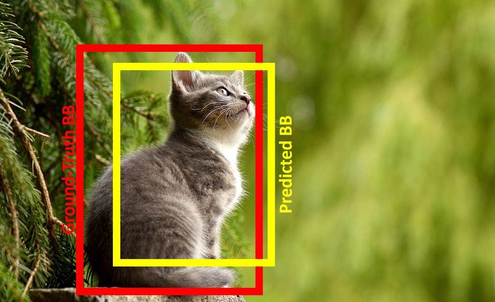
mAP (mean Average Precision) is a common metric used for evaluating the accuracy of object detection models. The mAP computes a score by comparing the ground-truth bounding box to the detected box. The higher the score, the more precise the model's detections.

The following articles give a good overview of the concepts of precision, recall, mAP, etc. 

https://jonathan-hui.medium.com/map-mean-average-precision-for-object-detection-45c121a31173

https://blog.paperspace.com/mean-average-precision/

https://blog.paperspace.com/deep-learning-metrics-precision-recall-accuracy/

https://www.narendranaidu.com/2022/01/confusion-matrix-for-classification.html

Some snippets from the above article:

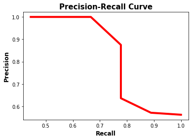
"When a model has high recall but low precision, then the model classifies most of the positive samples correctly but it has many false positives (i.e. classifies many Negative samples as Positive). When a model has high precision but low recall, then the model is accurate when it classifies a sample as Positive but it may classify only some of the positive sample.

Higher the precision, the more confident the model is when it classifies a sample as Positive. The higher the recall, the more positive samples the model correctly classified as Positive.

As the recall increases, the precision decreases. The reason is that when the number of positive samples increases (high recall), the accuracy of classifying each sample correctly decreases (low precision). This is expected, as the model is more likely to fail when there are many samples.

The precision-recall curve makes it easy to decide the point where both the precision and recall are high. The f1 metric measures the balance between precision and recall. When the value of f1 is high, this means both the precision and recall are high. A lower f1 score means a greater imbalance between precision and recall.

The average precision (AP) is a way to summarize the precision-recall curve into a single value representing the average of all precisions. The AP is the weighted sum of precisions at each threshold where the weight is the increase in recall. 

The IoU is calculated by dividing the area of intersection between the 2 boxes by the area of their union. The higher the IoU, the better the prediction.

The mAP is calculated by finding Average Precision(AP) for each class and then average over a number of classes."

Difference between Epoch, Batch and Iterations

In neural nets, we have to specify the number of epochs while we train the model. 

One Epoch is defined as the complete forward & backward pass of the neural net over the complete training dataset. We need to remember that Gradient Descent is an iterative process and hence we need multiple passes (or epochs) to find the optimal solution. In each epoch, the weights and biases are updated. 

Batch size is the number of records in one batch. One Epoch may consist of multiple batches. The training dataset is split into batches because of memory space requirements. A large dataset cannot be fit into memory all at once. With increase in Batch size, required memory space increases. 

Iterations is the number of batches needed to complete one epoch. So if we have 2000 records and a batch size of 500, then we will need 4 iterations to complete one epoch. 

If the number of epochs are low, then it results in underfitting the data. As the number of epochs increases, more number of times the weight are changed in the neural network and the curve goes from underfitting to optimal to overfitting curve. Then how do we determine the optimal number of epochs?

It is done by splitting the training data into 2 subsets - a) 80% for training the neural net  b) 20% for validating the model after each epoch. The fundamental reason we split the dataset into a validation set is to prevent our model from overfitting. The model is trained on the training set, and, simultaneously, the model evaluation is performed on the validation set after every epoch.

Then we use something called as the "early stopping method"-  we essentially keep training the neural net for an arbitrary number of epochs and monitor the performance on the validation dataset after each epoch. When there is no sign of performance improvement on your validation dataset, you should stop training your network. This helps us arrive at the optimal number of epochs. 

A good explanation of these concepts is available here - https://www.v7labs.com/blog/train-validation-test-set. Found the below illustration really useful to understand the split of data between train/validate/test sets. 

Ruminating on Convolutional Neural Networks

Convolutional Neural Nets (CNNs) have made Computer Vision a reality. But to understand CNNs, we need to get basics right - What exactly is a convolution? What is a kernel/filter?

The kernel or filter is a small matrix that is multiplied by the source image matrix to extract features. So you can have a kernel that identifies edges or corners of a photo. Then there could be kernels that detect patterns - e.g. eyes, stripes.

A convolution is a mathematical operation where a kernel (aka filter) moves across the input image and does a dot product of the kernel and the original image. This dot product is saved as a new matrix and is called as the feature map. An excellent video visualizing this operation is available here - https://youtu.be/pj9-rr1wDhM

Image manipulation software such as Photoshop also use kernels for effects such as 'blur background'. 

One fundamental advantage of the convolution operation is that if a particular filter is designed to detect a specific type of feature in the input, then applying that filter systematically across the entire input image allows us to discover that feature anywhere in the image. Also note that a particular convolutional layer can have multiple kernels/filters. So after the input layer (a single matrix), the convolutional layer (having 6 filters) will produce 6 output matrices. A cool application to visualize this is here - https://www.cs.ryerson.ca/~aharley/vis/conv/flat.html

A suite of tens or even hundreds of other small filters can be designed to detect other features in the image. After a convolutional layer, we also typically add a pooling layer. Pooling layers are used to downsize the features maps - keeping the important parts and discarding the rest. The output matrices of the pooling layer are smaller in size and faster to process. 

So as you can see, the fundamental difference between a densely connected layer and a convolutional layer is that dense fully connected layers learn global patterns (involving all pixels) whereas convolution layers learn local features (edges, corners, textures, etc.) 

Using CNNs, we can create a hierarchy of patterns - i.e. the second layer learns from the first layer. CNNs are also reusable, so we can take an image classification model trained on https://www.image-net.org/ dataset and add additional layers to customize it for our purpose. 

A good introduction to CNN models is given in this article - https://towardsdatascience.com/convolution-neural-networks-a-beginners-guide-implementing-a-mnist-hand-written-digit-8aa60330d022 with a good PyTorch implementation for MNIST dataset here - https://towardsdatascience.com/mnist-handwritten-digits-classification-using-a-convolutional-neural-network-cnn-af5fafbc35e9

Ruminating on Activation Function

 Activation functions play an important role in neural nets. An activation function transforms the weighted sum of the input into an output from a node. 

Simply put, an activation function defines the output of a neuron given a set of inputs. It is called "activation" to mimic the working of a brain neuron. Our neurons get activated due to some stimulus. Similarly the activation function will decide which neurons in our neural net get activated. 

Each hidden layer of a neural net needs to be assigned an activation function. Even the output layer of a neural net would use an activation function. 

The ReLU (Rectified Linear Unit) function is the most common function used for activation. 

The ReLU function is a simple function: max(0.0, x). So essentially it takes the max of either 0 or x. Hence all negative values are ignored. 

Other activation functions are Sigmoid and Tanh. The sigmoid activation function generates an output value between 0 and 1. 

An excellent video explaining activation function is here - https://youtu.be/m0pIlLfpXWE

The activation functions that are typically used for the output layer are Linear, Sigmoid (Logistic) or Softmax. A good explanation of when to use what is available here - https://machinelearningmastery.com/choose-an-activation-function-for-deep-learning/

Ruminating on Gradient Descent

Gradient Descent is the most popular optimization algorithm used to train machine learning models - by minimizing the cost function. In deep learning, neural nets use back-propagation that internally use a cost function (aka lost function) like Gradient Descent. 

The Gradient descent function essentially uses calculus to find the direction of travel and then to find the local minimal of a function. The following 2 videos are excellent tutorials to understand Gradient Descent and their use in neural nets. 

https://youtu.be/IHZwWFHWa-w

https://youtu.be/sDv4f4s2SB8

Once you understand these concepts, it will help you also realize that there is no magic involved when a neural net learns by itself -- ultimately a neural net learning by itself just means minimizing a cost function (aka loss function).

Neural nets start with random values for their weights (of the channels) and biases. Then by using the cost function, these hundreds of weights/biases are shifted towards the optimal value - by using optimization techniques such as gradient descent. 

Ruminating on 'Fitting the line to data'

 In linear regression, we need to find the best fit line over a set of points (data). StatQuest has an excellent video explaining how we fit a line to the data using the principle of 'least squares' - https://www.youtube.com/watch?v=PaFPbb66DxQ

The best fit line is the one where the sum of the squares of the distances from the actual points to the line is the minimum. Hence this becomes an optimization problem in Maths that can be calculated. We square the distances to take care of negative values/diffs. 

In stats, the optimization function that minimizes the sum of the squared residuals is also called as a 'loss function'. 

The equation of any line can be stated as: y = ax + b

where a is the slope of the line and b is the y-intercept. Using derivates we can find the most optimal values of 'a' and 'b' for a given dataset. 

Ruminating on CUDA and TPU

 CUDA  is a parallel computing platform (or a programming model - available as an API) that was developed by Nvidia to enable developers leverage the full parallel processing power of its GPUs. 

For deep learning (training neural nets) requires a humongous amount of processing power and it is here that HPCs with thousands of GPU cores (e.g. A100 GPU) are essential. 

Nvidia has also released a library for use in neural nets called as cuDNN. CUDA Deep Neural Network library (cuDNN) is a GPU-accelerated library of primitives for deep neural networks. cuDNN provides highly tuned implementations for standard routines such as forward and backward convolution, pooling, normalization, and activation layers.

Many deep learning frameworks rely on CUDA & the cuDNN library for parallelizing work on  GPUs - Tensorflow, Caffe2, H2O.ai, Keras, PyTorch. 

To address the growing demand for training ML models, Google came up with it's own custom integrated circuit called as TPU (Tensor Processing Unit). A TPU is basically a ASIC (application-specific integrated circuit) designed by Google for use in ML. TPU's are tailored for TensorFlow and can handle massive multiplications and additions for neural networks, at great speeds while reducing the use of too much power and floor space. 

Examples: Google Photos use TPU's to process more than 100 million photos every day. TPU's also power Google RankBrain - that part of Google's algorithm that uses machine-learning and artificial intelligence to better understand the intent of a search query. 

Understanding what is a Tensor?

Found this excellent video on YouTube by Prof. Daniel Fleisch that explains tensors in a very simple and engaging way - https://youtu.be/f5liqUk0ZTw

Tensors are are generalizations of vectors & matrices to N-dimensional space.

• A scalar is a 0 dimensional tensor
• A vector is a 1 dimensional tensor
• A matrix is a 2 dimensional tensor
• A nd-array is an N dimensional tensor

The inputs, outputs, and transformations within neural networks are all represented using tensors.  A tensor can be visualized as a container which can house data in N dimensions.

Ruminating on the Turing Test

 The Turing Test was made famous by Alan Turing in the year 1950. The Turing Test essentially tests a computer's ability to communicate indistinguishably from a human. The Turing Test was also called as the 'Imitation Game' by Alan earlier. 

A good introduction to the Turing Test can be found here - https://youtu.be/3wLqsRLvV-c

Though many claim that the turing test was passed by a AI chatbot called Eugene Goostman, but in reality it is not so. No computer has ever passed the Turing Test - https://isturingtestpassed.github.io/

Intelligent chatbots have really come a long way - The Google Duplex Demo e.g. https://youtu.be/0YaAFRirkfk

Maybe when we achieve AGI (Artificial General Intelligence), then the Turing Test would be accurately passed :)

Ruminating on n-gram models

N-gram is a fundamental concept in NLP and is used in many language models. In simple terms, N-gram is nothing but a sequence on N words - e.g. San Francisco (is a 2-gram) and The Three Musketeers (is a 3-gram). 

N-grams are very useful because they can be used for making next word predictions, correcting spellings or grammar. Ever wondered how Gmail is able to suggest auto-completion of sentences? This is possible because Google has created a language model that can predict next words.

N-grams are also used for correcting spelling errors - e.g. “drink cofee” could be corrected to “drink coffee” because the language model can predict that 'drink' and 'coffee' being together have a high probability. Also the 'edit distance' between 'cofee' and 'coffee' is 1, hence it is a typo.

Thus N-grams are used to create probabilistic language models called n-gram models. N-gram models predict the occurrence of a word based on its N – 1 previous word. 

The 'N' depends on the type of analysis we want to do - e.g. Research has also shown that trigrams and 4-grams work the best for spam filtering. 

Some good info on N-grams is available at the Standford University site - https://web.stanford.edu/~jurafsky/slp3/slides/LM_4.pdf

Google books also has a "N-Gram" viewer displays a graph showing how those phrases have occurred in a corpus of books (e.g., "British English", "English Fiction", "French") over the selected years. I found this to be useful in understanding what topic was popular in which years: https://books.google.com/ngrams

Ruminating on Text Normalization

Text normalization is the process of converting text to a standard form before we use them for training AI NLP models. The following techniques are typically used for normalizing text. 

Tokenization:  Tokenization is the process of breaking down sentences into words. In many Latin-derived languages, "space" is considered to be a word delimeter. But there are special cases such as 'New York', 'Rock-n-Roll' etc. Also Chinese and Japanese languages do not have spaces between words. We may laso wante to tokenize emoticons and hashtags. 

Lemmatization: In this process, we check if words have the same 'root' - e.g. sings, sang. We then normalize the words to the common root word. 

Stemming: Stemming can be considered a form of Lemmatization wherein we just strip the suffixes from the end of the word - e.g. troubled and troubles can be stemmed to 'troubl'.

Lemmatization is more computationally intensive than Stemming because it actually maps the word to a dictionary and finds the root word. Whereas Stemming just uses some crude heuristic process that chops off the ends of words in the hope of getting the root word. Stemming is thus much faster when you are dealing with a large corupus of text. The following examples will make the difference clear. 

• The word "better" has "good" as its lemma. This link is missed by stemming, as it requires a dictionary look-up.
• The word "walk" is the base form for word "walking", and hence this is matched in both stemming and lemmatisation.
• If you lemmatize the word 'Caring', it would return 'Care'. If you stem, it would return 'Car' and this is erroneous.

Sentence Segmentation: This entails breaking up a long sentence into smaller sentences using chars such as '! ; ?'. 

Spelling Correction and UK/US differences: As part of the normalization activity, we may also want to correct some common spelling mistakes and also normalize the different spelling between UK/US like neighbour/neighbor.

Ruminating on Fourier Transformation

 In my AI learning journey, I had to refresh my understanding of fourier transformation. The following video on YouTube is hands-down the best tutorial for understanding this maths concept.

Fourier transformations are used in AI Computer Vision models for usecases such as edge detection, image filtering, image reconstruction, and image compression.